This type of diagram was originally suggested and used by Keisler (1976a, 1976b), but not formalized by constructing optical lenses.
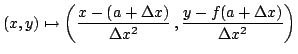
Let ![]() be a real function with continuous second derivative (
be a real function with continuous second derivative (![]() ). If we magnify
an infinitesimal neighborhood by a more powerful tool than an optical
). If we magnify
an infinitesimal neighborhood by a more powerful tool than an optical ![]() -lens, we can
see other interesting properties of the curve. This is what we call a microscope
``within'' a microscope pointed in
-lens, we can
see other interesting properties of the curve. This is what we call a microscope
``within'' a microscope pointed in
![]() in the non-optical
in the non-optical ![]() -lens
(because the optical lenses lose every infinitesimal details). By an optical
-lens
(because the optical lenses lose every infinitesimal details). By an optical ![]() -lens
pointed in
-lens
pointed in ![]() , both the curve
, both the curve ![]() and the tangent
and the tangent
![]() are
mapped in the line
are
mapped in the line
![]() , where
, where
![]() and
and ![]() is an
infinitesimal of the same order as
is an
infinitesimal of the same order as ![]() . Now we can put
. Now we can put
![]() and point a
and point a
![]() -lens in
-lens in
![]() . In order to visualize more details, we need to have
more information about the function: our idea is to use the non-standard Taylor's second
order formula for
. In order to visualize more details, we need to have
more information about the function: our idea is to use the non-standard Taylor's second
order formula for ![]() (see (Stroyan and Luxemburg, 1976)), i.e.
(see (Stroyan and Luxemburg, 1976)), i.e.
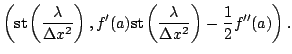
Thus the
![]() -lens maps as follows
-lens maps as follows
Therefore, we have
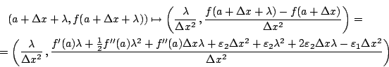
The point
![]() on the
graph of the tangent line is mapped in the point
on the
graph of the tangent line is mapped in the point
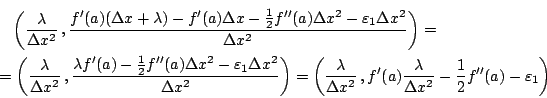
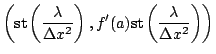
This suggests nice new (and mathematically justified, of course) mental representations
of the concept of tangent line: through the optical
![]() -lens, the tangent line can
be seen as the line
-lens, the tangent line can
be seen as the line
![]() which means that the graph of the
function and the graph of the tangent are distinct, straight, and parallel lines in a
which means that the graph of the
function and the graph of the tangent are distinct, straight, and parallel lines in a
![]() -neighborhood of
-neighborhood of
![]() . The fact that one line is either below or
above the other, depends on the sign of
. The fact that one line is either below or
above the other, depends on the sign of ![]() , in accordance with the standard real
theory: if
, in accordance with the standard real
theory: if ![]() is positive (or negative) in a neighborhood, then
is positive (or negative) in a neighborhood, then ![]() is convex (or
concave) here and the tangent line is below (or above) the graph of the function.
is convex (or
concave) here and the tangent line is below (or above) the graph of the function.
![\includegraphics[width=6cm]{c:/texdocs/conferences/html/micro2.eps}](img64.gif)